教學來源
https://satijalab.org/seurat/articles/pbmc3k_tutorial
本教學以 PBMC3K 資料為例,介紹 Seurat 進行單細胞 RNA 分析的完整流程。
1. 建立 Seurat 物件
 1# 清除環境變數,避免影響後續分析
 2rm(list = ls(all = TRUE))
 3
 4# 載入必要套件
 5library(dplyr)
 6##
 7## Attaching package: 'dplyr'
 8## The following objects are masked from 'package:stats':
 9##
10##     filter, lag
11## The following objects are masked from 'package:base':
12##
13##     intersect, setdiff, setequal, union
14library(Seurat)
15## Loading required package: SeuratObject
16## Warning: package 'SeuratObject' was built under R version 4.4.3
17## Loading required package: sp
18## Warning: package 'sp' was built under R version 4.4.2
19##
20## Attaching package: 'SeuratObject'
21## The following objects are masked from 'package:base':
22##
23##     intersect, t
24library(patchwork)
25## Warning: package 'patchwork' was built under R version 4.4.3
26library(ggplot2)
27## Warning: package 'ggplot2' was built under R version 4.4.3
28
29# 設定資料目錄並載入 10X 格式的資料
30setwd("C:/Users/TPOW31714/Desktop/20250224 Human microarray for CY_add cell/4. RDS/filtered_gene_bc_matrices/hg19/")
31data_dir <- "C:/Users/TPOW31714/Desktop/20250224 Human microarray for CY_add cell/4. RDS/filtered_gene_bc_matrices/hg19/"
32pbmc.data <- Read10X(data.dir = data_dir)
33
34# 建立 Seurat 物件,並過濾掉少於 200 個基因表現或出現在少於 3 個細胞的基因
35pbmc <- CreateSeuratObject(counts = pbmc.data, project = "pbmc3k", min.cells = 3, min.features = 200)
36## Warning: Feature names cannot have underscores ('_'), replacing with dashes
37## ('-')
38
39# 可選:轉換原始 count 矩陣與 metadata 為 data.frame 形式
40X1 <- pbmc@assays[["RNA"]]@layers[["counts"]] %>% as.data.frame()
41X2 <- pbmc@meta.data
2. 品質控制與細胞篩選
 1# 計算每個細胞的粒線體基因比例 (以 MT- 開頭的基因表示)
 2pbmc[["percent.mt"]] <- PercentageFeatureSet(pbmc, pattern = "^MT-")
 3
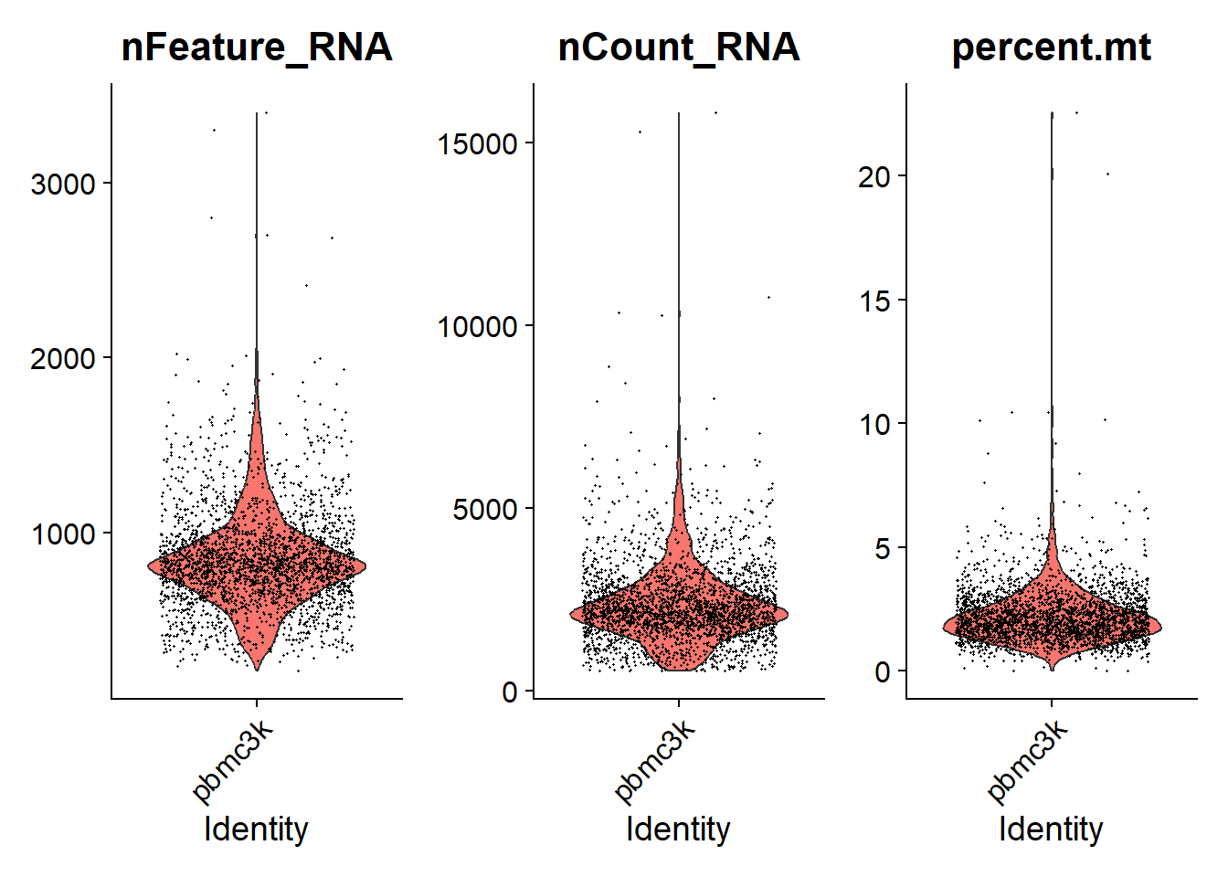
 4# 使用 VlnPlot 觀察 nFeature、nCount 與 percent.mt 分布
 5VlnPlot(pbmc, features = c("nFeature_RNA", "nCount_RNA", "percent.mt"), ncol = 3)
 6## Warning: Default search for "data" layer in "RNA" assay yielded no results;
 7## utilizing "counts" layer instead.
 8## Warning: The `slot` argument of `FetchData()` is deprecated as of SeuratObject 5.0.0.
 9## ℹ Please use the `layer` argument instead.
10## ℹ The deprecated feature was likely used in the Seurat package.
11##   Please report the issue at <https://github.com/satijalab/seurat/issues>.
12## This warning is displayed once every 8 hours.
13## Call `lifecycle::last_lifecycle_warnings()` to see where this warning was
14## generated.
15## Warning: `PackageCheck()` was deprecated in SeuratObject 5.0.0.
16## ℹ Please use `rlang::check_installed()` instead.
17## ℹ The deprecated feature was likely used in the Seurat package.
18##   Please report the issue at <https://github.com/satijalab/seurat/issues>.
19## This warning is displayed once every 8 hours.
20## Call `lifecycle::last_lifecycle_warnings()` to see where this warning was
21## generated.
1
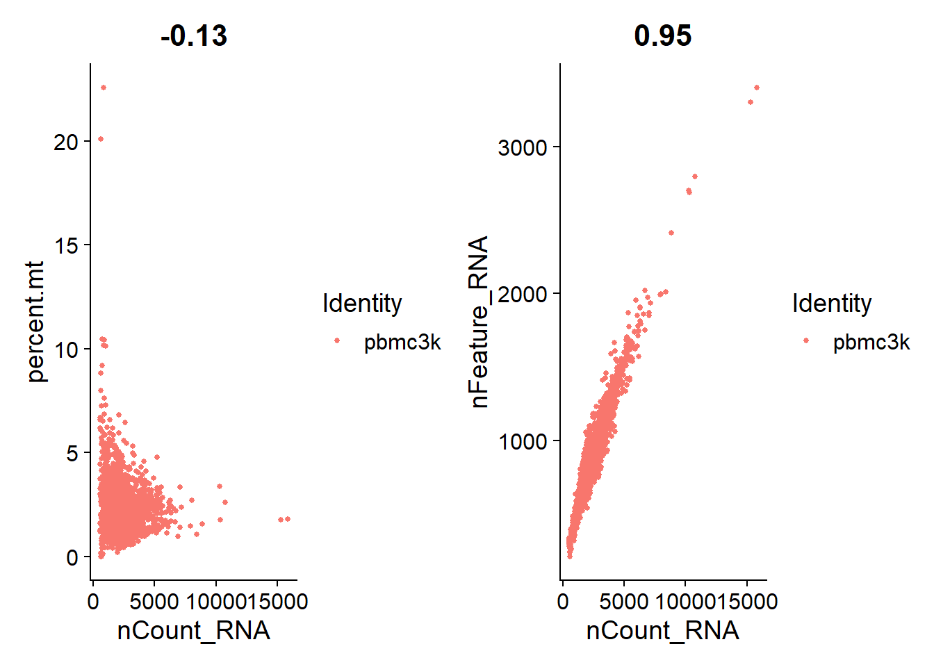
2# 使用 FeatureScatter 檢查 feature 之間的相關性
3plot1 <- FeatureScatter(pbmc, feature1 = "nCount_RNA", feature2 = "percent.mt")
4plot2 <- FeatureScatter(pbmc, feature1 = "nCount_RNA", feature2 = "nFeature_RNA")
5plot1 + plot2
1
2# 篩選細胞:去除少於 200 或大於 2500 基因表現 & 粒線體比例 > 5% 的細胞
3pbmc <- subset(pbmc, subset = nFeature_RNA > 200 & nFeature_RNA < 2500 & percent.mt < 5)
3. 正規化資料
1# 將每個細胞表現值進行 LogNormalize
2pbmc <- NormalizeData(pbmc, normalization.method = "LogNormalize", scale.factor = 10000)
3## Normalizing layer: counts
4
5# 轉出正規化後的資料矩陣
6X3 <- pbmc@assays[["RNA"]]@layers[["data"]] %>% as.data.frame()
4. 高變異基因篩選
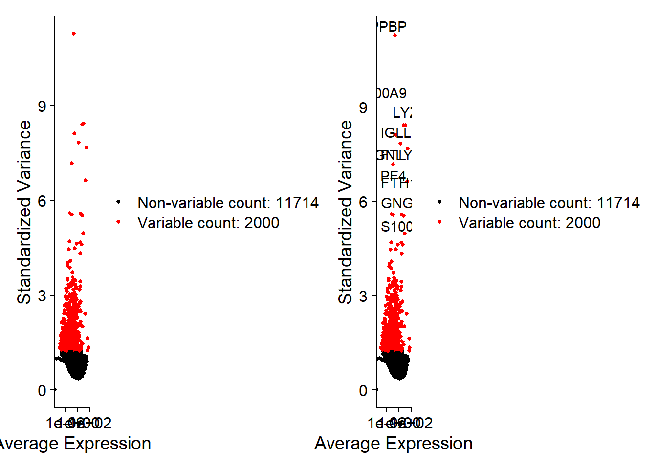
 1# 尋找 2000 個高變異基因 (用於 PCA 分析)
 2pbmc <- FindVariableFeatures(pbmc, selection.method = "vst", nfeatures = 2000)
 3## Finding variable features for layer counts
 4
 5# 顯示最變異的前 10 個基因
 6top10 <- head(VariableFeatures(pbmc), 10)
 7plot1 <- VariableFeaturePlot(pbmc)
 8plot2 <- LabelPoints(plot = plot1, points = top10, repel = TRUE)
 9## When using repel, set xnudge and ynudge to 0 for optimal results
10plot1 + plot2
11## Warning in scale_x_log10(): log-10 transformation introduced infinite values.
12## log-10 transformation introduced infinite values.
5. 資料標準化(scaling)
1# 對所有基因進行中心化與標準差轉換
2all.genes <- rownames(pbmc)
3pbmc <- ScaleData(pbmc, features = all.genes)
4## Centering and scaling data matrix
6. PCA 降維分析
 1# 使用高變異基因進行 PCA
 2pbmc <- RunPCA(pbmc, features = VariableFeatures(object = pbmc))
 3## PC_ 1
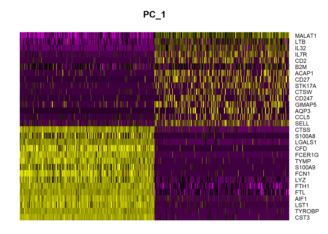
 4## Positive:  CST3, TYROBP, LST1, AIF1, FTL, FTH1, LYZ, FCN1, S100A9, TYMP
 5## 	   FCER1G, CFD, LGALS1, S100A8, CTSS, LGALS2, SERPINA1, IFITM3, SPI1, CFP
 6## 	   PSAP, IFI30, SAT1, COTL1, S100A11, NPC2, GRN, LGALS3, GSTP1, PYCARD
 7## Negative:  MALAT1, LTB, IL32, IL7R, CD2, B2M, ACAP1, CD27, STK17A, CTSW
 8## 	   CD247, GIMAP5, AQP3, CCL5, SELL, TRAF3IP3, GZMA, MAL, CST7, ITM2A
 9## 	   MYC, GIMAP7, HOPX, BEX2, LDLRAP1, GZMK, ETS1, ZAP70, TNFAIP8, RIC3
10## PC_ 2
11## Positive:  CD79A, MS4A1, TCL1A, HLA-DQA1, HLA-DQB1, HLA-DRA, LINC00926, CD79B, HLA-DRB1, CD74
12## 	   HLA-DMA, HLA-DPB1, HLA-DQA2, CD37, HLA-DRB5, HLA-DMB, HLA-DPA1, FCRLA, HVCN1, LTB
13## 	   BLNK, P2RX5, IGLL5, IRF8, SWAP70, ARHGAP24, FCGR2B, SMIM14, PPP1R14A, C16orf74
14## Negative:  NKG7, PRF1, CST7, GZMB, GZMA, FGFBP2, CTSW, GNLY, B2M, SPON2
15## 	   CCL4, GZMH, FCGR3A, CCL5, CD247, XCL2, CLIC3, AKR1C3, SRGN, HOPX
16## 	   TTC38, APMAP, CTSC, S100A4, IGFBP7, ANXA1, ID2, IL32, XCL1, RHOC
17## PC_ 3
18## Positive:  HLA-DQA1, CD79A, CD79B, HLA-DQB1, HLA-DPB1, HLA-DPA1, CD74, MS4A1, HLA-DRB1, HLA-DRA
19## 	   HLA-DRB5, HLA-DQA2, TCL1A, LINC00926, HLA-DMB, HLA-DMA, CD37, HVCN1, FCRLA, IRF8
20## 	   PLAC8, BLNK, MALAT1, SMIM14, PLD4, P2RX5, IGLL5, LAT2, SWAP70, FCGR2B
21## Negative:  PPBP, PF4, SDPR, SPARC, GNG11, NRGN, GP9, RGS18, TUBB1, CLU
22## 	   HIST1H2AC, AP001189.4, ITGA2B, CD9, TMEM40, PTCRA, CA2, ACRBP, MMD, TREML1
23## 	   NGFRAP1, F13A1, SEPT5, RUFY1, TSC22D1, MPP1, CMTM5, RP11-367G6.3, MYL9, GP1BA
24## PC_ 4
25## Positive:  HLA-DQA1, CD79B, CD79A, MS4A1, HLA-DQB1, CD74, HIST1H2AC, HLA-DPB1, PF4, SDPR
26## 	   TCL1A, HLA-DRB1, HLA-DPA1, HLA-DQA2, PPBP, HLA-DRA, LINC00926, GNG11, SPARC, HLA-DRB5
27## 	   GP9, AP001189.4, CA2, PTCRA, CD9, NRGN, RGS18, CLU, TUBB1, GZMB
28## Negative:  VIM, IL7R, S100A6, IL32, S100A8, S100A4, GIMAP7, S100A10, S100A9, MAL
29## 	   AQP3, CD2, CD14, FYB, LGALS2, GIMAP4, ANXA1, CD27, FCN1, RBP7
30## 	   LYZ, S100A11, GIMAP5, MS4A6A, S100A12, FOLR3, TRABD2A, AIF1, IL8, IFI6
31## PC_ 5
32## Positive:  GZMB, NKG7, S100A8, FGFBP2, GNLY, CCL4, CST7, PRF1, GZMA, SPON2
33## 	   GZMH, S100A9, LGALS2, CCL3, CTSW, XCL2, CD14, CLIC3, S100A12, RBP7
34## 	   CCL5, MS4A6A, GSTP1, FOLR3, IGFBP7, TYROBP, TTC38, AKR1C3, XCL1, HOPX
35## Negative:  LTB, IL7R, CKB, VIM, MS4A7, AQP3, CYTIP, RP11-290F20.3, SIGLEC10, HMOX1
36## 	   LILRB2, PTGES3, MAL, CD27, HN1, CD2, GDI2, CORO1B, ANXA5, TUBA1B
37## 	   FAM110A, ATP1A1, TRADD, PPA1, CCDC109B, ABRACL, CTD-2006K23.1, WARS, VMO1, FYB
38
39# 輸出 PCA 結果,檢視前 5 個主成分
40print(pbmc[["pca"]], dims = 1:5, nfeatures = 5)
41## PC_ 1
42## Positive:  CST3, TYROBP, LST1, AIF1, FTL
43## Negative:  MALAT1, LTB, IL32, IL7R, CD2
44## PC_ 2
45## Positive:  CD79A, MS4A1, TCL1A, HLA-DQA1, HLA-DQB1
46## Negative:  NKG7, PRF1, CST7, GZMB, GZMA
47## PC_ 3
48## Positive:  HLA-DQA1, CD79A, CD79B, HLA-DQB1, HLA-DPB1
49## Negative:  PPBP, PF4, SDPR, SPARC, GNG11
50## PC_ 4
51## Positive:  HLA-DQA1, CD79B, CD79A, MS4A1, HLA-DQB1
52## Negative:  VIM, IL7R, S100A6, IL32, S100A8
53## PC_ 5
54## Positive:  GZMB, NKG7, S100A8, FGFBP2, GNLY
55## Negative:  LTB, IL7R, CKB, VIM, MS4A7
56
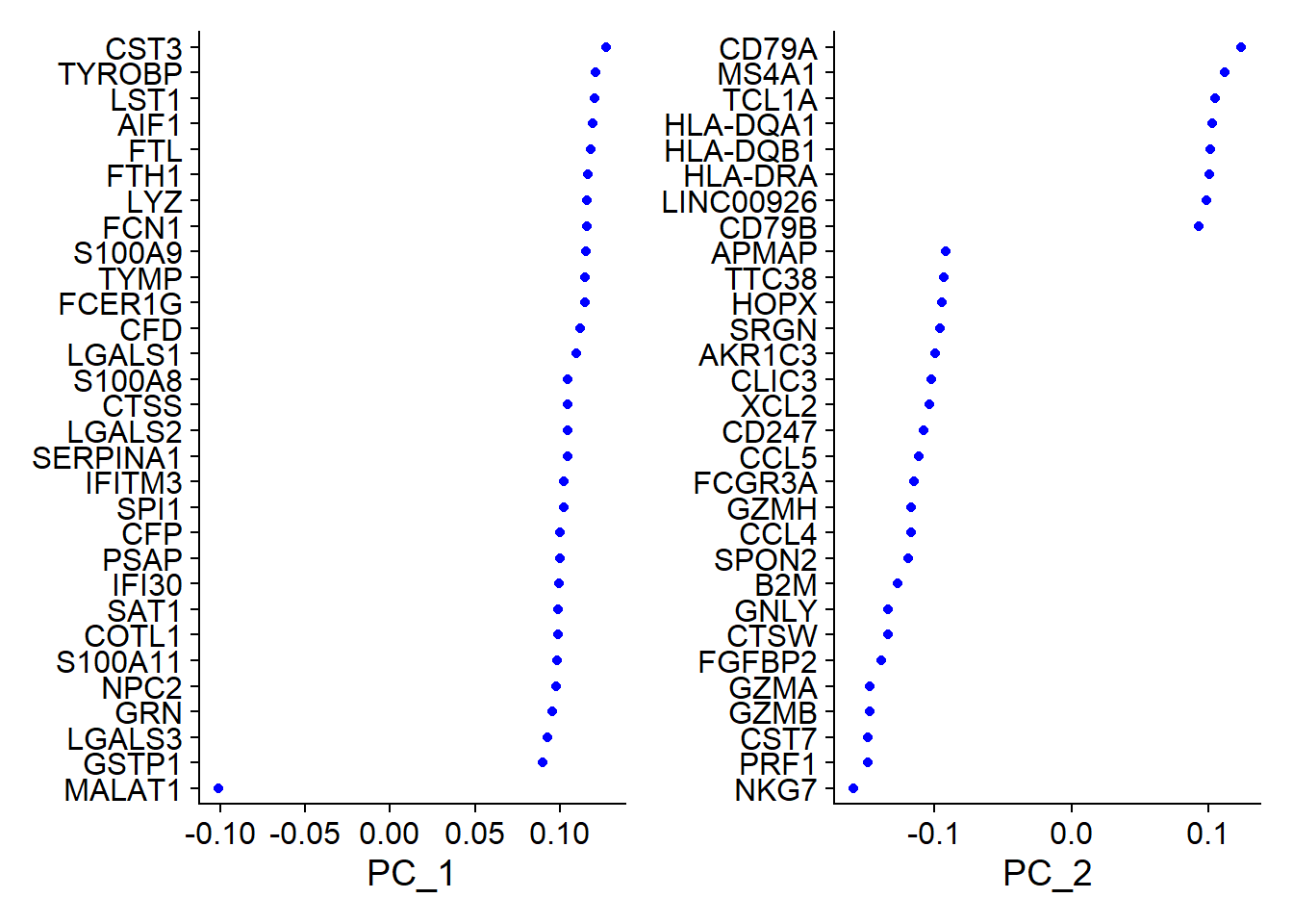
57# 顯示載重圖、降維圖與熱圖
58VizDimLoadings(pbmc, dims = 1:2, reduction = "pca")
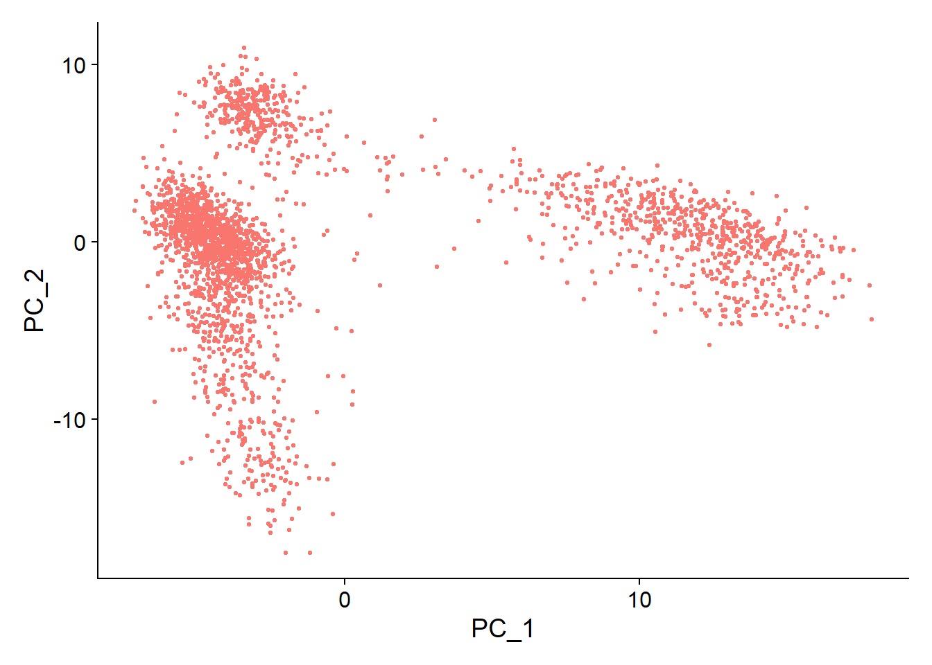
1DimPlot(pbmc, reduction = "pca") + NoLegend()
1DimHeatmap(pbmc, dims = 1, cells = 500, balanced = TRUE)
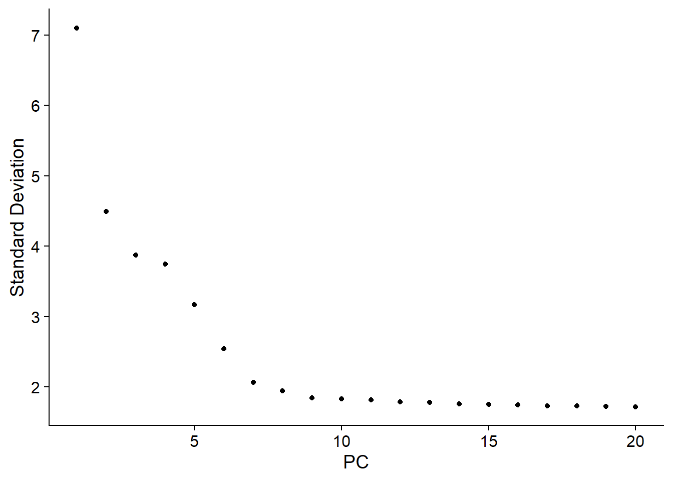
7. 選擇最佳維度數量(Elbow Plot)
1ElbowPlot(pbmc)
8. 建立近鄰圖與群集分析
 1pbmc <- FindNeighbors(pbmc, dims = 1:10)
 2## Computing nearest neighbor graph
 3## Warning: package 'future' was built under R version 4.4.3
 4## Computing SNN
 5pbmc <- FindClusters(pbmc, resolution = 0.5)
 6## Modularity Optimizer version 1.3.0 by Ludo Waltman and Nees Jan van Eck
 7##
 8## Number of nodes: 2638
 9## Number of edges: 95927
10##
11## Running Louvain algorithm...
12## Maximum modularity in 10 random starts: 0.8728
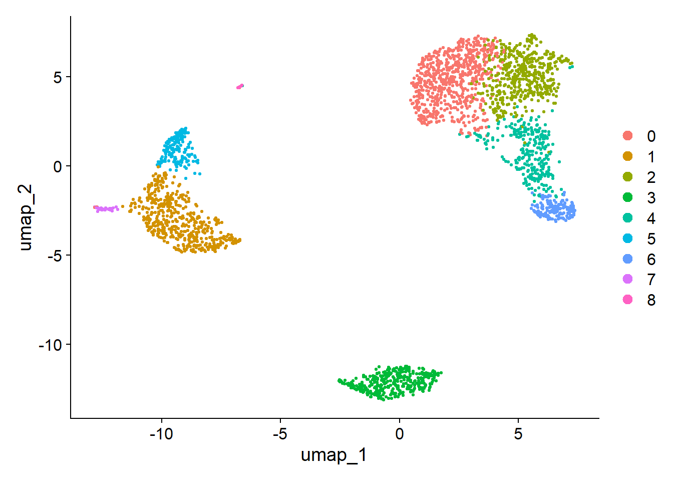
13## Number of communities: 9
14## Elapsed time: 0 seconds
9. 非線性降維:UMAP
 1pbmc <- RunUMAP(pbmc, dims = 1:10)
 2## Warning: The default method for RunUMAP has changed from calling Python UMAP via reticulate to the R-native UWOT using the cosine metric
 3## To use Python UMAP via reticulate, set umap.method to 'umap-learn' and metric to 'correlation'
 4## This message will be shown once per session
 5## 19:27:19 UMAP embedding parameters a = 0.9922 b = 1.112
 6## 19:27:19 Read 2638 rows and found 10 numeric columns
 7## 19:27:19 Using Annoy for neighbor search, n_neighbors = 30
 8## 19:27:19 Building Annoy index with metric = cosine, n_trees = 50
 9## 0%   10   20   30   40   50   60   70   80   90   100%
10## [----|----|----|----|----|----|----|----|----|----|
11## **************************************************|
12## 19:27:20 Writing NN index file to temp file C:\Users\TPOW31~1\AppData\Local\Temp\RtmpM1mnaL\file74a4f381b69
13## 19:27:20 Searching Annoy index using 1 thread, search_k = 3000
14## 19:27:20 Annoy recall = 100%
15## 19:27:20 Commencing smooth kNN distance calibration using 1 thread with target n_neighbors = 30
16## 19:27:21 Initializing from normalized Laplacian + noise (using RSpectra)
17## 19:27:21 Commencing optimization for 500 epochs, with 105140 positive edges
18## 19:27:21 Using rng type: pcg
19## 19:27:26 Optimization finished
20DimPlot(pbmc, reduction = "umap")
1
2# 儲存結果
3saveRDS(pbmc, file = "pbmc_tutorial.rds")
10. 差異表現基因分析
 1# cluster 2 與其他 cluster 的差異表現基因
 2cluster2.markers <- FindMarkers(pbmc, ident.1 = 2)
 3## Warning: The `slot` argument of `GetAssayData()` is deprecated as of SeuratObject 5.0.0.
 4## ℹ Please use the `layer` argument instead.
 5## ℹ The deprecated feature was likely used in the Seurat package.
 6##   Please report the issue at <https://github.com/satijalab/seurat/issues>.
 7## This warning is displayed once every 8 hours.
 8## Call `lifecycle::last_lifecycle_warnings()` to see where this warning was
 9## generated.
10
11# cluster 5 與 cluster 0 與 3 的差異
12cluster5.markers <- FindMarkers(pbmc, ident.1 = 5, ident.2 = c(0, 3))
13
14# 全部 cluster 的 marker gene
15pbmc.markers <- FindAllMarkers(pbmc, only.pos = FALSE)
16## Calculating cluster 0
17## Calculating cluster 1
18## Calculating cluster 2
19## Calculating cluster 3
20## Calculating cluster 4
21## Calculating cluster 5
22## Calculating cluster 6
23## Calculating cluster 7
24## Calculating cluster 8
25pbmc.markers_1 <- pbmc.markers %>% group_by(cluster) %>% filter(avg_log2FC > 1)
26write.table(pbmc.markers, "pbmc_Findallmarkers_250610.txt", sep = "\t", row.names = TRUE)
27
28# 使用不同檢定法,例如 ROC
29cluster0.markers <- FindMarkers(pbmc, ident.1 = 0, test.use = "roc", only.pos = TRUE)
30
31# 可視化 marker gene
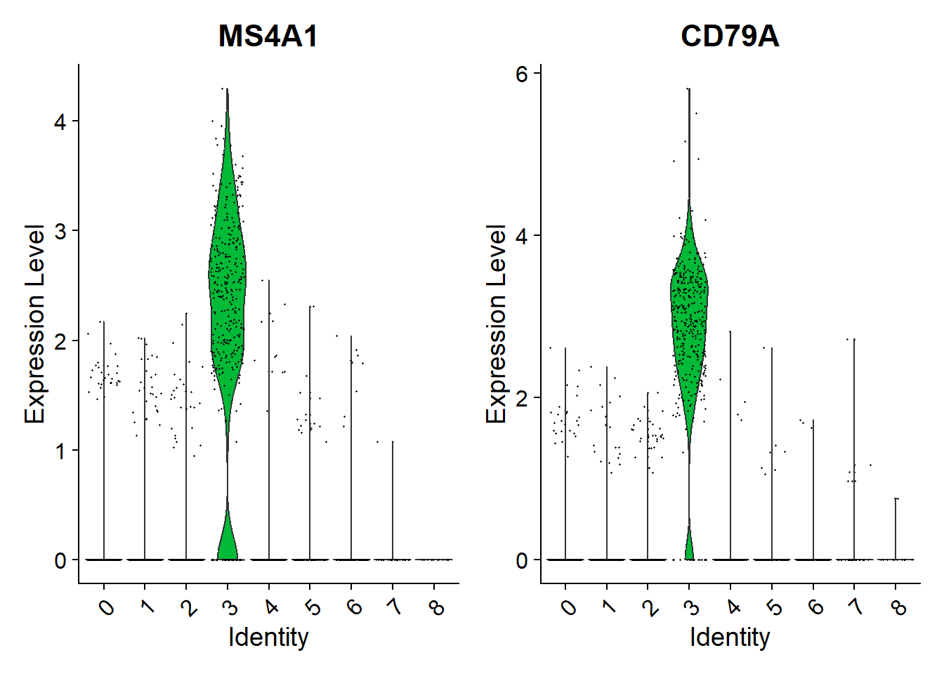
32VlnPlot(pbmc, features = c("MS4A1", "CD79A"))
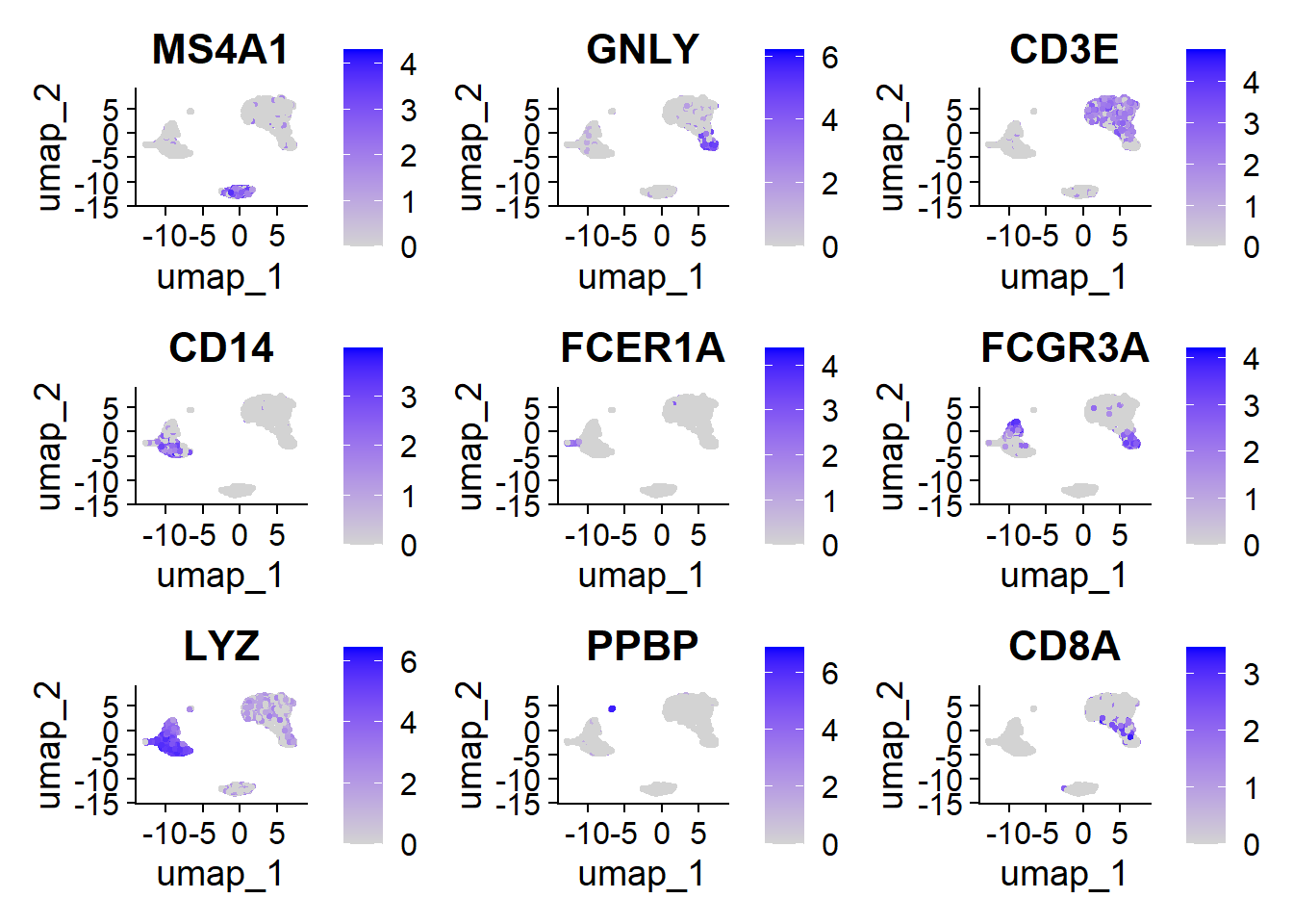
1FeaturePlot(pbmc, features = c("MS4A1", "GNLY", "CD3E", "CD14", "FCER1A", "FCGR3A", "LYZ", "PPBP", "CD8A"))
1
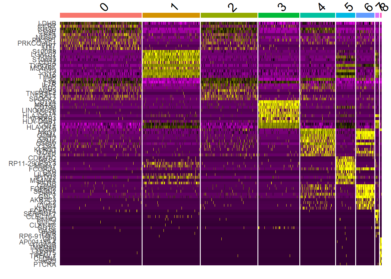
2# 熱圖顯示每群前 10 個基因
3top10 <- pbmc.markers %>% group_by(cluster) %>% filter(avg_log2FC > 1) %>% slice_head(n = 10)
4DoHeatmap(pbmc, features = top10$gene) + NoLegend()
11. 命名各群細胞類型
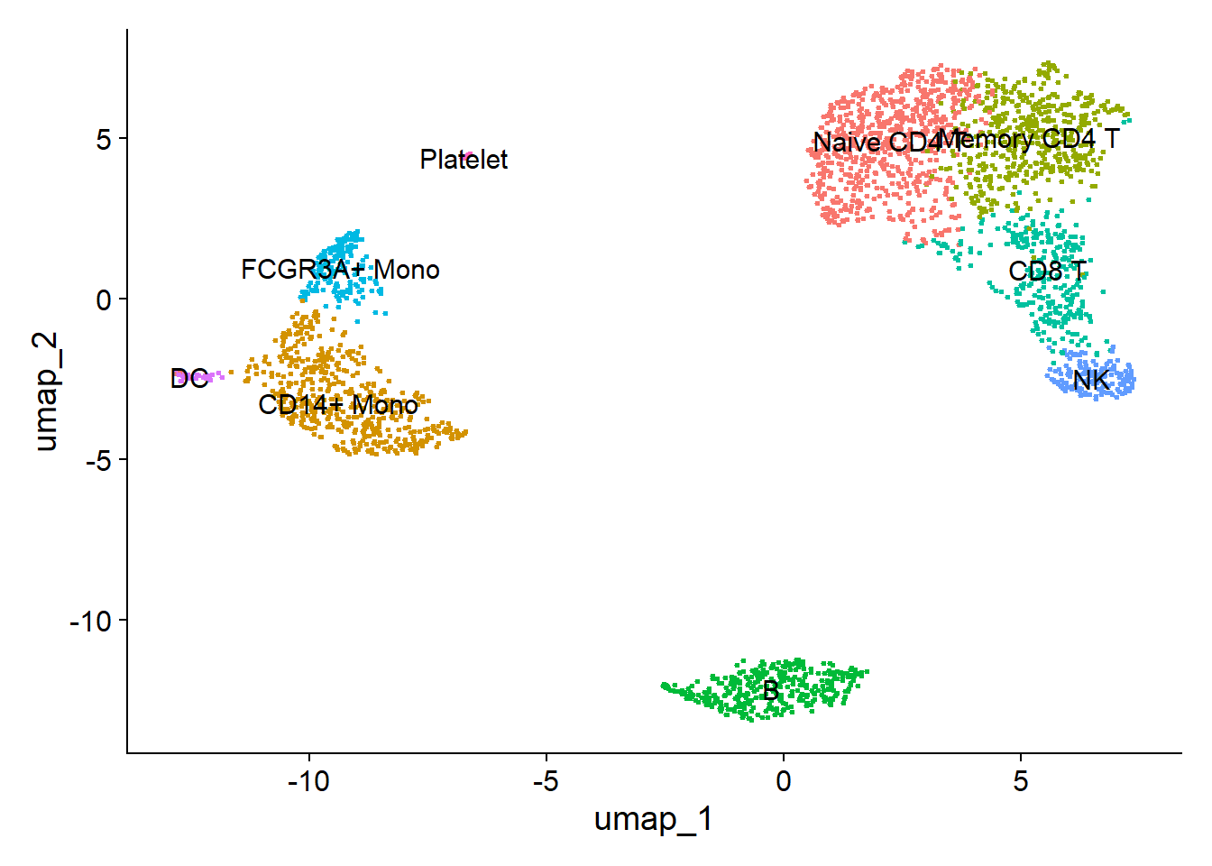
1new.cluster.ids <- c("Naive CD4 T", "CD14+ Mono", "Memory CD4 T", "B", "CD8 T", "FCGR3A+ Mono", "NK", "DC", "Platelet")
2names(new.cluster.ids) <- levels(pbmc)
3pbmc <- RenameIdents(pbmc, new.cluster.ids)
4
5# 畫出標註細胞類型的 UMAP 圖
6DimPlot(pbmc, reduction = "umap", label = TRUE, pt.size = 0.5) + NoLegend()
1
2# 儲存高解析圖檔
3plot <- DimPlot(pbmc, reduction = "umap", label = TRUE, label.size = 4.5) +
4  xlab("UMAP 1") + ylab("UMAP 2") +
5  theme(axis.title = element_text(size = 18))
6
7ggsave(filename = "pbmc3k_umap.jpg", height = 7, width = 12, plot = plot)
更多視覺化方法請參考官方文件:https://satijalab.org/seurat/articles/visualization_vignette
補充說明:PCA vs UMAP 原理與差異
PCA(主成分分析)
- 線性降維方法,將高維基因資料轉換成具有最大變異的主成分。
- 優點:計算快速、結果可解釋性高。
- 缺點:無法處理非線性資料結構。
UMAP(統一流形近似與投影)
- 非線性降維方法,以保留資料的局部鄰近關係為目標。
- 優點:適合視覺化高維度 scRNA-seq 資料。
- 缺點:結果有隨機性,較難直接解釋每個軸的生物意義。
比較表格
| 項目 | PCA | UMAP |
|---|---|---|
| 類型 | 線性降維 | 非線性降維 |
| 解釋性 | 高 | 低 |
| 運算速度 | 非常快 | 中等 |
| 是否保留全域結構 | 是 | 否,偏向保留局部結構 |
| 結果穩定性 | 穩定 | 不穩定(需 set.seed 固定) |
| 適合視覺化 | 一般 | 非常適合 |
| 常見用途 | 降維前處理、選擇維度 | UMAP 聚類圖、轉錄軌跡圖 |
在 Seurat 中的建議用途:
- PCA 用於決定
FindNeighbors()和FindClusters()使用的維度數量。 - UMAP 主要用於可視化細胞的分群與異質性。
Comments